 Machine learning (ML) is the heart of AI products (Alexa, Siri, Cortana, Driverless Car etc.), algorithms are the core component of ML and mathematics is brain behind these algorithms. While data scientists can build model without requiring to deep dive into the underlying mathematics, but model performance with variability of data/information might be limiting until we have good grip & understanding about algorithms, its characteristics, parameters and tenet. Seasoned Data Scientists (DS) select appropriate algorithm (viz. Logistics Regression, RNN, Decision Tree, PCA, NMF, Random forest, naïve-bayes and many other) along with its parameters values (regularization, learning rate, gaussian width etc.) to build model depending upon business case, problem statement and available training data. Such abilities are developed with very good foundation of mathematics (Primarily Linear Algebra, calculus and statistics) and its application while designing and/or using algorithm. Academicians have produced a slew of algorithms and its quite accessible through various libraries (Scikit-Learn, TensorFlow, H20, MLib-Spark etc.). While we understand different roles and related fields in AI (read my earlier blog), let’s put good deal of effort to understand underlying math to embrace the journey of becoming a good data scientist or ML engineer. I will write few posts about some of widely used ML algorithm (Primarily in BFSI domain) while explaining mathematics behind the same, use cases and codes in Python. In this blog, I have picked up SVM (Support Vector Machine) and may need 3-4 posts in sequence to keep quality and quantity balanced.
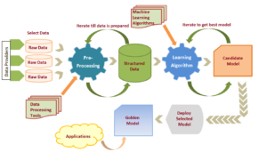
SVM is one of many well practiced and quite an evolving supervised machine learning models and can be used for both classification and regression problems. SVM has evolved from maximum margin classifier (focusing to maximize the separation margin) to kernel trick (effective way of drawing non-linear classifier) to soft margin kernelized classifier (use regularization to reduce overfitting). We will clarify all that in next few posts in the order of (a) General intuition about SVM (b) Underlying mathematics and (c) Kernel implementation to solve complex classification problems (e.g. Non-linear classifier). There are numerous use cases and product built around SVM such as alert fraudulent transactions, classify bad assets/loans, classify auto drivers into aggressive, average and very simple for Insurance risk profile purpose, and many more. Approximately 70% of modeling effort goes into data engineering & preparation work such as data extraction, cleansing, labeling, normalizations, data access control, quantification etc. before we start applying ML (Machine Learning model) such as SVM (SVC or SVR for classification or Regression respectively) upon data to train the model. Like many other top ML Models, SVM involves quite a daunting and intense mathematics.
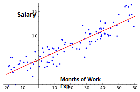
Use intuition to understand ML Mathematics: One should take help of intuition before coming under the grinding wheel of mathematics. It’s easy to visualize linear or logistic regression involving 2 to 3 coordinates/parameters resulting into a line or plane as models. So, let’s visualize or understand intuitively till 3D, beyond that let mathematics encounter the situation and our job will be easier to understand the algorithm. For ex. We gathered sample data from Industries and found that, as work experience increases, salary increases (Visualize a straight line but may be with huge OLS – Ordinary Least Square error, meaning work exp. is not only deciding the salary) so , we add another parameter to justify salary, say no. of certificates, and then higher studies, and then work locations, and so on until we don’t get relevant parameters/features that can add information to the learning and thereby obtain minimal error. We can visualize a straight line, then a plane and that’s it, beyond that it would hyperplane that can’t be easily visualized. But we have got the intuition that work exp., certificates, etc. are influencing the value of salary. If we can build mathematical equation involving couple of parameters, we can as well extend to any number of parameters and this is what we going to learn in SVM model.
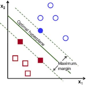
What is SVM with an example: Let’s take bunch of emails as set of data points as an example for binary classification problem. Problem statement: Build a classifier to flag SPAM email and move them into spam folder!!! We need training and test data set to build machine learning model, so we read and label emails either ‘genuine’ or ‘spam’ email as 0 or 1 (label and data point values must always be numeric). An SVM algorithm (from library package e.g. – Scikit-learn , TensorFlow, mahout etc.) reads these labeled data points/emails (Supervised means we have created a labeled data points to train a model) and learns to classify futuristic emails . Hypothetically, the SVM trained model draws a line or plane or hyperplane (depending upon number of features of emails) to separate between ‘genuine’ and ‘spam’ emails. So, SVM is ML model that involves associated algorithms to create line/plane/hyperplane by learning from training dataset and builds a classifier or regressor (model) to classify futuristic data points into one of the many classes. Separator/classifier could be linear or non-linear. SVM model builds the hyperplane that is the maximum from nearest training datapoints from all classes. This important characteristic of maximum margin classifier yields less generalization error for such SVM model. (It’s easy to imagine in a binary classification in the picture shown below).
Involved Mathematics: SVM Goal is to Identify the optimal hyperplane (line or plane or hyperplane for 2D,3D or multi D features) with maximum margin between nearest training datapoints (nearest datapoints are Support Vectors, pic.)
Before I get into full mathematics, let me get the list of basics mathematics, equations and formula that will be required in deriving the optimal hyperplane. SVM packages use the same mathematics internally and renders classifiers as values of coefficients and bias after learning from data points (or after running against training labeled dataset).
- Linear Algebra: In a 3D scenario, equation of plane is AX+BY+CZ=D , and its norm will be (A, B, C) coordinate We can convert equation into general vector yet condensed form as W*X+b = 0 (Where W∈(W1,W2,W3…) is weight or Coefficient vectors , X = feature or coordinate variables set ∈(X,Y,Z…) and b= bias constant. This equation can be applicable to line, plane or hyperplane but we can’t visualize beyond 3D so lets math take care of representation and calculations.
- Vector calculations : Refresh with some calculations such as unit vector n ̂ = (A ⃗ /mod(A)), distance from a point to the plane (calculate normal [⟂] of the plane => project data point vector to the normal (dot product) and take magnitude), vector additions, dot products etc.
- Calculus – refer 10+2 standard on differentiation, partial differentiation and double differentiation, best is to refer khan academy. This small calculus will be used for determining minimum or maximum points in a function. As we learned earlier, critical points of a function will have f’(x,y) = 0 and f’’(x,y) sign (+ => Minima, – => maxima) . (Cond. Function must be continuous else we wouldn’t be able to double diff.).
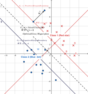
Margin is the distance between two planes and our goal is to find maximum margin (Pic. above): –
- data set => We have two classes of samples, Class 1 (Red star) and Class 2 (Blue Dots)
- Each sample has two features (X and Y axis), so this is 2-Dimensional set
- We draw 2 lines in parallel coinciding with at least one data point from each class at their respective boundary (RED line for C1 and Blue line for C2)
- After that draw a line in parallel to both boundary lines in the middle (dotted line) =>C0
- We will try to make this dotted line as an ideal classifier while keeping the margin both the sides. The goal is to keep margin maximum so that futuristic data points get less generalization error.
Now we have hyperplane equation, and with the help of above picture, basic linear algebra concepts and few research outcome (Convex function, Lagrange multiplier, KKT (Karush-Kuhn-Ticker) validation) we can derive optimal hyperplane. I will keep this topic for next few blogs and will try to explain in simple and intuitive way. In the meanwhile, please send comment/feedback and happy reading until the next edition!!!