Support Vector Machine : Part 2 (Build intuition before applying mathematics)

As discussed in previous part, we continue building intuition before jumping into its (SVM) underlying mathematics. Please read previous part before reading this post. Our goal is to find the optimal hyperplane (it could be line, plane or hyperplane depending upon number of features or parameters) i.e. the hyperplane which is having the maximum distance from data points of each class. (please refer to fig. in previous part)

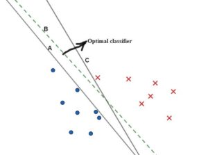
Let’s try to visually identify which one of the classifiers is optimal from the fig. A, B or C. B (dotted line) looks reasonably well since it is almost middle of both type of data points. For simplicity sake, we take a collection of data points (or data set) which is linearly separable (Linearly separable – A linear line can be drawn between two types of data, e.g. one type is complaint call and other type appreciation call, let’s say we are trying to build a classifier to analyze customer call) and we will build a linear classifier (model) that classifies futuristic customer call into one of these. We have taken only two features (in X/Y plane) for the sake of explanation and ease of visualization (In real world it could be many more such features such as tone pitch(high freq. audio clip), words, length of call, words frequency etc.) . Let’s say blue is call with appreciation and red with complaint. From the picture we can estimate the one having the maximum distance from both classes. The optimal model builds such maximum margin classifier as the optimal hyperplane because it would have some reasonably good margin (It’s always safer to allow few spills over data elements through these margins and yet not get mis-classified) created along with the ability to classify futuristic data correctly.

But, how do we find such optimal classifier. It is not easy to draw a separator having tons of features in realistic business scenario, such as emails(you can’t draw hyperplane with several features such as words dictionary), so mathematics is the savior here that helps determine optimal hyperplane. We will go in steps as described below while referring to the same 2D graph to understand mathematics.

We have plotted data points in XY plane and gave different color (red and blue) for type of data set (One type could SPAM email – Red and other Genuine email – Blue). We are not taking all features but only two features data set (for the same of easy visualization) presuming it is linear separable.

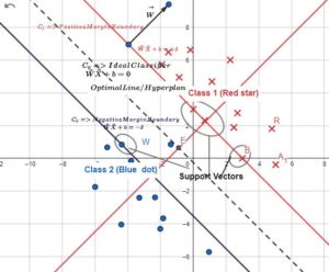
Equation of a line: mx+ny+p= 0, in xy plane. or mx₁+nx₂+p=0 in x₁, x₂ plane, where x₁ and x₂ are features/parameters.
As discussed in the previous post, We convert this equation to vector form as WX+b=0 where (W=[w1,w2]=[m, n], X=[ x₁, x₂],b=-p/n where W is the vector perpendicular to the line. We can extend this formula to any number of parameters of axes, and we will have the same concept for W (or $\overrightarrow{W}$ ), which is the vector with coordinate [w1, w2, w3…wn] and is perpendicular to the hyperplane.
So our classifier is f(w,b) = WX+b, W and b are variables that change the line or classifier orientation. For a given W and b, we can check the sign of data points. (X is not a variable but actual data point coordinates, given W and b, for a particular coordinate of data point, we obtain one value)
Let’s draw a parallel and equidistant lines from main classifier, their equations are $\overrightarrow{W}\overrightarrow{X}+b=+\delta$ and $\overrightarrow {W}\overrightarrow {X}+b=-\delta$ . Basically any points above mid line will be +ve, on the mid line will be 0 and below will be -ve. These 2 parallel lines have same W but b & δ can be adjusted to keep margins as appropriate as can be. For simplicity we make δ =1 (we can scale these values for calculation simplification)

Calculate Margin: (m) We will use vector calculation :-

HP (hyperplane) equations with X0 and X1 points become WX₁+b=1 and WX₀+b=-1
X1=X_o+k = X0+mW/|W| (Letter in bold is in vector form)
Hyperplane equation with X1 point => WX₁+b = 1
W(Xo+mW/|W|)+b=1
(WX₀+b)/|W|+mW*W/|W|=1
Substituting WX₀+b = -1 (above equation) => mW²/|W|=2
m= 2/|W|

So, margin m is inversely proportional to vector W, but what does this mean?

m (Margin) between 2 HPs can be maximized when W, which is the vector perpendicular to HPs, is minimized.

Optimization Problem: Our goal is to find the maximum margin or minimum W. At what value of W and b, margin equation gets us the maximum value, is nothing but Optimization Problem. While we try to find the min W, we have to maintain the constraint of keeping all data points beyond margins. This can be addressed using optimization function, and mathematically we can write as below: –

$\begin{aligned}\min _{\left| \omega \right| }f\left( \omega \right) \\ s.t.\ \overrightarrow {W}\cdot \overrightarrow {X_i}+b\geq 1 for\ y_{i }=+1\ and \\ \overrightarrow {W}\cdot \overrightarrow {X_i}+b\leq -1\ for\ y_{i }=-1 \end{aligned}$

We can combine both constraints into one as below. We multiply the marginal expression with label, so combined expression $y_{i}( \overrightarrow {W}\cdot \overrightarrow {X_i}+b)\geq 1$ will always be positive for all i , i.e $\forall i\in \left( 1\ldots n\right)$

Here f(w) = W and we want to find minimum W under given constraint.

We can transform the function (f) from W to , which still holds true for finding minimum w. (min w is equivalent to min $\dfrac {1}{2}W^{2}$ , since this expression will be easier to differentiate.

Lagrange multiplier and Lagrange equation:- As we know from the 10+2 standard, we take derivative to obtain min or max value of a function. We call ‘gradient’ as term for derivative if number of variables are greater than 1. So, the expression f’(x) = 0 means, we get the value of x for which f’ is 0. If the function is constrained by another function/s then we combine parent function with all other constraining functions by multiplying constraining functions with a set of multipliers and that is called Lagrange multiplier. The resultant expression is called Lagrangian Expression.

Example:-

$\begin{aligned}f\left( x\right) =x^{2}+3x+5 \\ g\left( x\right) =2x+1\geq 0 \\ h\left( x\right) =x+3 <0\end{aligned}$

Lagrangian expression = $L\left( x\right) =f\left( x\right) -\alpha _{1}g\left( x\right) -\alpha _{2}h\left( x\right)$

Intuitively we determine a point or coordinate where all functions derivatives/gradients (which are vectors) are equal. So above set of equation can be formalized as Lagrange equation as below: –

$\begin{aligned}f\left( w\right) =\dfrac {1}{2}\left\| W^{2}\right\| \\ g_{i}\left(w,b\right) =y_{i}\left( \overrightarrow {W}\cdot \overrightarrow {x}+b\right) -1\geq 0,\\ \forall i\in \left( 1\ldots n\right) \end{aligned}$

After putting through Lagrangian function:-

$L\left( \omega ,b,\alpha \right) =\dfrac {1}{2}\left\| W^{2}\right\| -\sum ^{m}_{i=1}\alpha _{i}\ast g_{i}\left( \overrightarrow {W},b\right)$

$L\left( \omega ,b,\alpha \right) =\dfrac {1}{2}\left\| W^{2}\right\| -\sum ^{m}_{i=1}\alpha _{i}\ast \left[ y_{i}\left( \overrightarrow {W}\overrightarrow {X}+b\right) -1\right]$

L = Lagrangian function with three variables (w, b and α), here α is Lagrange multiplier. m = no of data elements, Objective function is $\dfrac {1}{2}\left| W\right| ^{2}$

Now we take differentiation of L (lagrangian) function to obtain minimum value. Since we have more than 1 variables, we call it gradient with symbol as $\Delta$ else we could have used $\dfrac {dy}{dx}$

Duality: Since we have good number of data points, solving for w and b will be tedious using Lagrangian theorem so we will switch to the dual form. Optimization problem can be solved by either determining minimal value of objective(primal) function or maximum of the dual function. Please read for Duality (if interested to go further into research done by academics). Now we form the equation involving dual variables (Lagrange variable) as below:-

min max L(w,b,α)

(w,b) (α)

such that α_i >= 0 for i = ( 1,2,…n – all data points)

Above expression means, we take minimum value w.r.t w and b (Primal variables in minimization problem) and maximum value w.r.t α (dual variable in maximization dual expression) at the same time.

As derived above, Lagrangian expression becomes

$L\left( x\right) =\dfrac {1}{2}\left\| W^{2}\right\| -\sum ^{m}_{i=1}\alpha _{i}\ast \left[ y_{i}\left( \overrightarrow {W}\overrightarrow {X}+b\right) -1\right]$ ——–(A)

We solve for minimization problem (gradient w.r.t W and b to 0):-

$\nabla _{w}L=W-\sum ^{n}\alpha _{i}y_{i}x_{i}=0$ – – – — (1) (gradient of L w.r.t W, As mentioned before, notation is for gradient, which differentiation w.r.t multiple parameters, here W is a vector = [w1, w2…])

$\dfrac {\delta L}{\delta b}=-\sum ^{m}_{i=1}\alpha _{i}y_{i}=0$ ——— (2) (derivative of L w.r.t b)

After substituting W in (A) , we transform the Lagrangian equation to Wolf-dual and use notation as W:-

$W\left( b,\alpha \right) =\dfrac {1}{2}\left(\sum^{m}_{i=1}\alpha_{i}y_{i}x_{i}\right)\left(\sum^{m}_{j=1}\alpha_{j}y_{j}x_{j}\right)-\sum ^{m}_{i=1}\alpha_{i}\ast \left[ y_{i}\left( \left( \sum ^{m}_{j=1}\alpha _{j}y_{j}x_{j}\right) x_{i}+b\right) -1\right]$

After combining (A) , (1) and (2) and carrying out adequate cancellation we arrive at the expression below. We have successfully transformed the equation with one variable of α.

$\begin{aligned}W\left( \alpha \right) =\max \left( \sum ^{m}_{i=1}\alpha _{i}-\dfrac {1}{2}\sum ^{m}_{i=1}\sum ^{m}_{j=1}\alpha _{i}\alpha _{j}y_{i}y_{j}x_{i}x_{j}\right) \\ \alpha _{i} >0\forall i\in \left( 1\ldots m\right) \end{aligned}$

We have transformed by replacing w and b variables with α, and this is Wolfe dual Lagrangian function. We can see each data element has gone through inter lagrangian multiplier. Since Lagrangian formula works with equality, and we have inequality situation (all data points must be greater than or less than ). We have to meet the requirement of KKT (Karush-Kuhn-Tukcker) requirement to satisfy inequality condition. (I won’t be covering KKT condition in this article, so please read out material here if interested)

Now, we have the Lagrange Multipliers (α), what next!!!

After solving Wolf equation above W(α), we obtain vector α (all Lagrange multipliers) for which W(α) is maximum. So we have α (vector with all Lagrange Multiplier, same number as Data).

Evaluate W: Our goal has been to find out W (vector perpendicular to the hyperplane) and b.

From equation (1) above $W^{\cdot }=\sum ^{m}{i=1}\alpha {i}y_{i}x_{i}$ , We know α, and x_i, y_i are data points and their labels, so we can derive W!!!

Evaluate b: We know all data points near margin. At margin, we have $y_{i}\left( \overrightarrow {W}\overrightarrow {X}+b\right) =1$ , so $b=y_{i}-\overrightarrow {W}\overrightarrow {X}$ . We obtain hyperplane by putting w and b into the hyperplane equation (w.x+b).

Conclusion: In the summary, we developed equation for hyperplane (in 2D the hyperplane is a line, in 3D its plane and so on) in vector form. On further, we derived margin equation. With the help of Lagrangian and Wolf equation we transformed lagrangian (primal parameter equations) to single variable Wolf equation that helped to get us optimal value of alpha where function value is the highest. This whole of mathematics implementation is to derive hyperplane as optimal classifier that SVM algorithm calculates by going through all data points. Now, the above mathematics doesn’t complete the entire range of SVM variations. There has been great deal of improvisation in calculating b, w, deriving soft-margin, non-linear classifier etc. My point here is to embrace the mathematics behind any ML algorithm while building ML models for AI solution. Model description and its interpretation are becoming the need in regulatory domain primarily in BFSI domain. As we know that most of ML models are like black-box. However, while applying ML algorithm to build a model, one must be aware of underlying mathematics that helps in describing and interpreting the model to the regulators to a larger extent. I hope this post gives some sense of embracing mathematics and its need while learning or applying ML algorithms in solving business problems. I will be publishing SVM kernel mechanism to build non-linear classifier in one of the next blogs. Please send me your comments or questions !!!

Support Vector Machine : Part 2 (Build intuition before applying mathematics)